Revista del Centro de Investigación de la Unviersidad La Salle
Vol. 12, No. 45, enero-junio, 2016: 37-70
DOI: 10.26457/recein.v12i45.838

Flow of multiparticle collision dynamics fluids confined by physical barriers

Arturo AYALA-HERNÁNDEZ¹, Humberto HÍJAR²

¹Universidad La Salle Ciudad de México (México)
²Universidad La Salle Ciudad de México (México)

Correspondance author: humberto.hijar@lasallistas.org.mx

Received: octubre de 2015 | Accepted: marzo de 2016 |

Copyright © 2017 "Arturo AYALA-HERNÁNDEZ & Humberto HÍJAR." This is an open access article distributed under the Creative Commons Attribution License, which permits unrestricted use, distribution, and reproduction in any medium, provided the original work is properly cited.

Abstract

---

In the last years, Multiparticle Collision Dynamics (MPC) has become a major computational tool that allows for simulating fluids with properties closely resembling those of a physical fluid. Recently, we have introduced a methodology for confining MPC fluids in complex geometries based on the use of explicit forces (Ayala-Hernandez and Híjar, 2016). In this work, we extend this method in order to simulate flow in a slitlike geometry. This is achieved by introducing two solid parallel plane surfaces consisting of particles that interact with the particles of the MPC fluid by means of explicit repulsive forces. We test the applicability of the proposed technique in simulations of fluids confined between these parallel planes and subjected to a uniform force field. We find that our model yields the correct plane Poiseuille flow expected from hydrodynamics with slip boundary conditions. We carry out a large amount of numerical experiments in which the simulations parameters are varied in a wide range, in order to measure important quantities characterizing the flow and the fluid-solid interaction, e.g., the slip at the solid boundary and the effective viscosity of the fluid. Finally, we determine the conditions for which plane Poiseuille flows with stick boundary condition can be simulated

Keywords: Computational techniques in fluid dynamics, Laminar flows, Multiparticle Collision Dynamics, Molecular Dynamics.

Multiparticle Collision Dynamics (MPC) is a simulation technique introduced by Malevanets and Kapral (1999; 2000), that has been proved to be a very useful method for studying diverse systems of soft condensed matter (Yeomans, 2006; Kapral, 2008; Gompper et al, 2009). Some adventages of MPC that make it so appealing for the simulation of complex fluids are summarized as follows. Fisrt, MPC is based on particles and, consequently, can be combined with Molecular Dynamics (MD) (Frenkel and Smith, 2002; Griebel et al, 2007) in the study of systems where dissipative time and length-scales coexist with microscopic scales, e.g., colloids and polymer solutions (Padding and Louis, 2004; Ali et al, 2004; Hecht et al, 2005; Padding and Louis, 2006). Second, the MPC algorithm is stochastic and gives rise to the proper hydrodynamic fluctuations and Brownian forces (Yeomans, 2006; Padding and Louis, 2004; Híjar and Sutmann, 2011). Third, MPC is relatively simple and very stable over long-time simulations. Fourth, it has been succesfully described analytically from the stand points of the kinetic theory and the projection operator technique (Tüzel et al, 2003; Ihle and Kroll, 2001, 2003, Pooley and Yeomans, 2005, Gompper et al., 2009).

Thus, in summary, MPC constitutes a powerful mesoscopic simulation method, for which an excellent understanding has been achieved. Some applications of MPC include the simulation of colloids and polymers (Malevanets and Kapral, 2000; Padding and Louis, 2004, Kikuchi et al, 2002), of polymers under flow (Yeomans, 2006; Malevanets and Yeomans, 1999; Ripoll et al, 2004), of flow around objects (Lamura et al., 2001; Allahyarov and Gompper, 2002), of vesicles under flow (Noguchi and Gompper, 2005), of particle sedimentation (Jordá et al, 2010, 2012), and of tracking control of colloidal particles immersed in steady shear flows (Híjar, 2013; Fernández and Híjar, 2015; Híjar, 2015).

Despite of the success that MPC has had, it should be mentioned that in most of the studied cases, MPC fluids are assumed to extend ad infinitum, a situation that in practice is approximated by imposing periodic boundary conditions. In this context, it is still an uncompleted task to find a general procedure to impose spatial constraints on the motion of fluids simulated by MPC. Diverse authors have achieved the confinement of MPC fluids by supplementing the simulation with the so-called bounce-back boundary conditions, which simply reflect the incoming particles back into the bulk system, and are in some sense equivalent to impose the presence of hard walls (Malevanets and Kapral, 1999; Inoue et al, 2002; Jordá et al, 2010; Withmer and Luijten, 2010). A comparison of the performance of some of these confining methods based on such hard walls can be found in (Withmer and Luijten, 2010). Some fundamental issues that have been introduced in that reference concern procedures that can be followed to simulate the presence of moving walls, and quiescent and mobile surfaces with partial slip boundary conditions. More recently, the modifications in the stress tensor produced by the interaction of the MPC particles with reflecting walls have been rigorously calculated for confinement in a slit geometry with a simple shear in (Winkler and Huang, 2009). The analysis carried out there, has yielded a properly modified form of the MPC algorithm in the presence of walls that prevents any surface slip of the confined fluid and allows for simulating the correct plane Couette velocity profile.

More recently, we have proposed an alternative procedure for simulating restrictive boundary conditions in MPC in which physical walls are explicitely considered by means of interaction potentials yielding forces on the MPC particles (Ayala-Hernández and Híjar, 2016). We have been able to obtain a closed expression for these forces, which could be integrated in a completely similar fashion as the equations of motion are integrated in hybrid MD-MPC schemes. Using this procedure we have simulated cylindrical Poiseuille flow of MPC fluids (Ayala-Hernández and Híjar, 2016) and observed the correct hydrodynamic flow between two coaxial cylinders (Híjar and Ayala-Hernández, 2016; Ayala 2016). These kind of force-based boundary conditions, could be preferable to those imposed by hard walls from the physical point of view since they are closer to simulate the situation encountered in real systems, where fluid-solid interactions always arise from laws of force.

With the pursue of demostrating the analysis of the effects that force-based boundary conditions have on MPC fluids, we will consider another application of the method introduced in (Ayala-Hernández and Híjar, 2016), namely, the simulation of plane Poiseuille flow between two parallel planes, a problem that has been considered by diverse authors since the introduction of MPC. In their pioneering work, Malevanets and Kapral implemented the simulation of two-dimensional plane Poiseuille flow with MPC, in order to demonstrate the general viability of the algorithm (Malevanets and Kapral, 1999). Simulations of two-dimensional Poiseuille flow of MPC fluids were subsequently carried out in (Lamura et al., 2001). In these two cases, flow was forced through the twodimensional geometry by allowing particles within a specific region to have an average velocity coinciding with the analytical expression at the collision step. Simulations of threedimensional Poiseuille flow using MPC were first reported in (Allahyarov and Gompper, 2002), where flow was promoted by the application of an explicit field of force. The authors supplemented their method with a simple rescaling thermostat to avoid viscous heating. Subsequent analysis of plane Poiseuille flow in MPC (Huang et al., 2010; Withmer and Luijten, 2010; Imperio et al., 2011), have also considered the approach based on direct forces and thermostats. An excellent comparison of these methods is presented in (Bolintineanu et al., 2012) where it can be appreciated that details in the simulation technique could produce rather large modifications in the simulated flow. For instance, the use of different thermostats (Huang et al., 2015) could produce effective variations in the viscosity of the fluid, and the implementation of different boundary conditions could yield diverse degrees of slip at the confining walls. We will notice that our method based on explicit fluid-solid interactions will exhibit some drawbacks similar to those present in the aforementioned works. However, we will show that in the limit in which the MPC dynamics is dominated by interparticle collisions, our methodology yields flows that match very well the analytical expression.

We will also notice that our method will face some difficulties that are also present in simulations of MPC fluids constrained by hard walls. These difficulties are, mainly, the need for incorporating virtual particles in partially empty cells at the collision step, and the problem of removing partial slip at the confining walls. We will carefully discuss the way in which our method can be addapted to reproduce the correct velocity profile with no-slip boundary conditions in the case of a slit geometry. It is important to stress that the problem to be addressed, lies within a more general context in which the use of explicit forces could yield the simulation of MPC fluids in complex geometries, as it has been discussed in detail in (Ayala-Hernández, 2016). From a methodological point of view, it sounds plausible to test the viability of the method in simple situations first and, subsequently, in more complicated cases. The purpose of the present analysis is, precisely, to demonstrate that the method based on forces is valid to simulate a simple flow, that is well understood and can be analyzed from fluid mechanics for very well defined situations. In further publications, we will progressively study the applicability of this technique in cases of increasing geometric complexity (Ayala-Hernández, 2016; Híjar and Ayala-Hernández, 2016).

This paper is organized as follows. In section 2 we will present the expression for the confinement force exerted by an even plane surface on the MPC particles, which will be used subsequently in our simulations. In section 3 we will discuss the details about our numerical implementation. In section 4 we will present the results obtained from a large number of numerical experiments of simulation of plane Poiseuille flow. Finally, in Section 5 we will state our conclusions, and summarize the advantages and limitations of our approach.

As it was mentioned in section 1, MPC is a simulation method based on particles. All the particles of a usual MPC fluid are assumed to have the same mass, 𝑚, and to have positions and velocities that are continuous functions of time. Let us consider an ensemble consisting of 𝑁 such particles, moving in the presence of a physical wall. An expression for the force that the wall exerts on the MPC constituents has been derived under the assumption that it consists of a continuous surface distribution of particles, which interact with the MPC particles via the generalized Weeks-Chandler-Andersen (WCA) potential (Hansen and McDonald, 1986).

where $\underset{R}{\rightarrow}$ and $\underset{R^{'}}{\rightarrow}$ ′ represent, respectively, the position vectors of an MPC particle and a wall particle,ε is the interaction strength, σ is the effective diameter of the interaction, n is a positive integer, and $\tilde{\sigma}=\frac{1}{2^{6n}\sigma}$ is the cutoff radius of the interaction. It is important to mention that the WCA potential has been previously used in diverse studies to describe the interaction of MPC particles with solid suspended particles (Malevanets and Kapral, 1999; Hecht et al, 2005; Híjar, 2013).

In the limiting case in which the curvature of the surface is not significant, the expression for the interaction potential between the wall and the MPC particle located at $\underset{R}{\rightarrow}$ , reads as (Ayala-Hernandez and Híjar, 2015).

where $\underset{R^{*}}{\rightarrow}$ is the closest point on the surface to the position $\underset{R}{\rightarrow}$ , and ρ_s is the numerical surface density of particles at the wall.

Moreover, in the same limiting case, the force exerted by the wall on the particle located at $\underset{R}{\rightarrow}$ was shown to be

Therefore, in such approximation MPC particles are considered to interact with a wall that at the local level is a plane with normal parallel to $\underset{R}{\rightarrow}-\underset{R^{*}}{\rightarrow}$.

It can be seen that with the intention of getting a closed expression for this force, an analytical function $\underset{R^{*}}{\rightarrow}\left ( \underset{R}{\rightarrow} \right )$ must be given, which dependes on the specific geometry of the confining wall. Such a function can be obtained in some particular cases, when the geometry of the confining wall is not too intricate. One important case is the one corresponding to a plane wall, which will be, indeed, the case to be studied in section 3. Before we proceed with this application, it will be important to emphasize that since [Eq. 2] and [Eq. 3] give rise to purely repulsive forces, they can be used to simulate only surfaces with slip boundary conditions. This can be readily seen for the particular case of a plane wall, schematically illustrated in Fig. 1 (a), for which $\underset{F}{\rightarrow}$ points in the normal direction to the surface. In this case, the wall will act as a smooth surface since any incoming particle colliding with it will be reflected back into the bulk system with reversed momentum along the normal vector but unchanged tangential momentum.

The effects produced by rough surfaces can be incorporated in the description by including a force contribution parallel to the wall. In simulations, the easiest and most intuitive way to include such tangential contributions is to apply forces in the opposite direction to that of the velocities of the incoming particles. In our description, this procedure could be equivalent to produce local imperfections, in such a way that any MPC particle that enters into the interaction region defined by a surface coinciding with the original wall, will face a local barrier whose orientation depends on the particle's velocity. This situation is schematically illustrated in Fig. 1 (b). In this case, the force applied on the particle could be of the form $\underset{F}{\rightarrow}_{-v}=-F\left ( \underset{R}{\rightarrow} \right )\hat{\upsilon}_{in}$, where $F\left ( \underset{R}{\rightarrow} \right ) $ is the magnitude of the force given by [Eq. 2] and [Eq. 3], and 𝑣̂in is the unitary vector representing the incoming velocity. Since this force is conservative, the velocity of the particle after the interaction with the wall will be simply reverted and it could be anticipated that this procedure will yield results similar to those obtained from the application of the simple bounce-back rule, which indeed produces surfaces with partial slip. This will be shown to be the case in section 4. Hereafter, this procedure for obtaining fluid-solid interactions will be referred as the simulation scheme I.

In this way, with the purpose of obtaining fluid-wall interactions satisfying no slip boundary conditions, it will be necessary to add an extra tangential force, $\underset{F}{\rightarrow}_{||}$ , to that given in scheme I. This force must vanish if the particle is not in contact with the wall and its magnitude must be tuned to make it able to eliminate the slip at the surface. In the following, the interaction between the wall and the MPC particles that is achieved by the application of a total force $\underset{F}{\rightarrow}=\underset{F}{\rightarrow}_{-v}+\underset{F}{\rightarrow}_{||}$, will be referred as the scheme II, which is illustrated in Fig. 1 (c). If the magnitude of $\underset{F}{\rightarrow}_{||}$ is small with respect to $\underset{F}{\rightarrow}\left ( \underset{R}{\rightarrow} \right )$, this scheme will be equivalent to add a supplementary local inclination to the wall faced by the incoming particles.

In principle, $\underset{F}{\rightarrow}_{||}$ could be determined by calculating the stress tensor generated at the surface by its application, e.g., by means of a kinetic theory model for the MPC dynamics (Belushkin et al, 2011). Here, we will not perform such calculation, but, obtain $\underset{F}{\rightarrow}_{||}$ empirically from the results of a large number of simulation experiments of MPC fluids driven by a uniform force between two fixed parallel planes. It is worth mentioning that similar procedures, in which fluid-solid interactions are supplemented with additional tangential surface forces, have been employed also in MD simulations of particles in the presence of physical barriers (Pivkin and Karniadakis, 2005; Spijker et al., 2008). For MPC simulations, this work is the first one in which the effects of such forces are analyzed.

In summary, the three simulation schemes illustrated in Fig. 1, could be used to simulate flow with boundary conditions that include total slip (a), partial slip (b), and no-slip (c). In the present paper we will only consider cases (b) and (c).

Three procedures of implementing fluid-wall interactions in MPC. (a) Forces $\underset{F}{\rightarrow}$ (blue arrows), are applied in the normal direction to the surface defining the wall. (b) Scheme I: forces are applied against the incoming velocities of the particles (thin dashed lines). (c) Scheme II: an additional force, $\underset{F}{\rightarrow}_{||}$ , is applied in the direction of the surface.

In order to test the performance of the previous models, we conducted a series of simulations in which MPC fluids, constituted by N point particles of mass m, are confined between two parallel plane walls. A scheme of the simulated system is shown in Fig. 2, where it can be appreciated that the particles of the confining walls were distributed in two planes located at positions $x=\pm\left ( \tilde{\sigma}+L_x/2 \right )$. Accordingly, the interaction surfaces were located at $x=\pm L_x/2$. The lengths of the simulated system along the y and z directions were L_y and L_z , respectively.

It can be seen from these definitions that the pure phase of the fluid, i.e., the set of MPC particles that were not in contact with the wall particles, occupied a total volume L_xL_yL_z . An external uniform field was considered to be present which exerted a force per unit mass $\underset{g}{\rightarrow}=g\hat{e}_{z}$ on the fluid particles in the pure phase.Observe that, in a general context, the field $\underset{g}{\rightarrow}$ could result from a uniform pressure grandient acting on the fluid and, if the parallel planes are properly oriented, from the gravitational field.

Schematic illustration of the simulated system. This figure also shows the implementation used to introduce virtual particles.

The system evolved in time according to a hybrid scheme combining MD and MPC. On the one hand, MD allowed us to simulate the behavior of the fluid particles at the microscopic time-scale and took care of their interaction with the confining walls. On the other hand, MPC considered the interaction between the fluid particles in a coarse-grained fashion allowing us to incorporate collective effects occurring at the hydrodynamic time-scales. Due to the presence of the confining walls, our hybrid MD-MPC simulation scheme had particular features that do not appear in usual implementations. These features will be discussed in detail below.

Typical MD-MPC simulations proceed in two main steps, commonly referred as the streaming step and the collision step. During streaming, the positions and velocities of the MPC particles are updated according to an MD integration method, e.g., the velocity Störmer-Verlet method applied on a short time step of size $\Delta t_{\textrm{MD}}$ (Griebel et al, 2007). Consequently, if vectors $\underset{R}{\rightarrow}_i$ and $\underset{v}{\rightarrow}_i$ , for i = 1,2, … , N, are used to represent the positions and velocities of the MPC particles, in our algorithm they were updated according to

and

where $\underset{F}{\rightarrow}_{i}$ denotes the total force on the i-th particle. This force was calculated by adding the confining force given by [Eq. 2] and [Eq. 3], and the external force field $\underset{g}{\rightarrow}$ . For completeness, we present here the explicit form of the forces $\underset{F}{\rightarrow}_{i}$ used in our simulations. They were obtained for the particular case of confinement by the plane surfaces described at the beginning of this section, and in the case in which $\underset{g}{\rightarrow}$ is only applied on the particles in the pure MPC phase. They read as

where L_i is the distance penetrated by the ith MPC particle in the region of interaction with the wall, in the direction of its incoming velocity, $\underset{v}{\rightarrow}_{\textrm{in},i}$. Notice that [Eq. 6] applies for the simulation scheme II, while for the scheme I the same equation can be applied with F_||= 0. In the hybrid MD-MPC procedure, the characteristic collision step of MPC is applied at regular time intervals of size $\Delta t = n_{\textrm{MD}} \Delta t_{\textrm{MD}}$, i.e., after performing n_MD steps of the streaming integration method. In the usual implementation, also referred as Stochastic Rotation Dynamics (SRD) (Yeomans, 2006; Kapral, 2008; Gompper et al, 2009), the simulation box is subdivided into cells of volume a ³ , where interparticle collisions are simulated. With this purpose, the center of mass velocity of each cell is calculated and particles within the same cell are forced to change their velocities according to the rule

where $\underset{v}{\rightarrow}_{i}^{'}$ and $\underset{v}{\rightarrow}_{i}$ are the velocities of the ith particle after and before collision, respectively; $\underset{v}{\rightarrow}_{\textrm{c.m.}}$ is the center of mass velocity of the cell; and $R(\alpha ; \hat{n})$ is a stochastic rotation matrix, which rotates velocities by an angle 𝛼 around a random axis $\hat{n}$. It is worth stressing that α is a parameter whose value is fixed through the whole simulation, while $\hat{n}$ is sampled in each cell at every collision step by randomly selecting a point on the surface of a sphere with unit radius.

Physically, α is the angle at which the velocities of the MPC particles that happen to be at the same MPC cell at the collision step are rotated. Accordingly, it represents the degree of interaction between MPC particles and should not be confused with the angle at which MPC particles collide with the solid walls. As it has been shown by diverse authors (Malevanets and Kapral 1999; Malevanets and Kapral 2000; Pooley and Yeomans, 2005; Gompper et al., 2009), α determines the value of the transport coefficients of the simulated fluid. Therefore, simulations carried out with different values of α, represent numerical experiments with different fluids.

In order to preserve the property of Galilean invariance, a uniform random displacement of the collision cells was implemented, before collisions take place (Ihle and Kroll, 2001, 2003). In the presence of confining surfaces, this random displacement procedure has important implications for various aspects of MPC. In our case, without the random displacement, the boundary cells coincide with the solid planes. However, when displacement occurs, the cells at the bottom and top of the simulation box get partially empty and the subsequent collisions inside them will take place in a fluid with modified density, thus yielding different physical properties than in the interior cells (Winkler and Huang, 2009). In favor of restoring the numerical density at the boundary, virtual particles can be introduced that appear in the partially empty cells only at the collision step. With the purpose of incorporating such phantom particles, we follow a procedure similar to that introduced in (Winkler and Huang, 2009), by including an additional collision cell below the lower plane. Then, the whole collision cells are displaced in the positive x-direction by a uniform vector with components uniformly distributed within the range $[-a/2, a/2]$. Afterwards, the partially empty cells are filled with virtual particles. The number of such particles at a given cell, N_v, is determined by the number of fluid particles, N_f , in the boundary cell cut off by the opposite plane, as it is schematically illustrated in Fig. 2. In this manner, the average particle density is restored and the probability distribution for observing a given number of particles at the collision cells is preserved (Winkler and Huang, 2009).

It should be remarked that the collisional contribution to the stress tensor depends on the velocity of the virtual particles. More precisely, it can be shown that the momentum exchanged in a collision cell between fluid and virtual particles, after averaging over fluctuations and stochastic rotations, reads as (Winkler and Huang, 2009)

where $\underset{v}{\rightarrow}_{\textrm{f}}$𝑣 f and $\underset{v}{\rightarrow}_{\textrm{v}}$ represent the average velocity of the fluid and virtual particles, respectively. In this work, we decided to incorporate the virtual particles with a velocity equals to the center of mass velocity of the partially empty layer in which they collide. Consequently, in our implementation we have $\underset{v}{\rightarrow}_{\textrm{f}} = \underset{v}{\rightarrow}_{\textrm{v}}$, and this procedure will not modify the stress at the boundary wall due to collisions

It should be also punctuated that if particles interacting with the confining walls ($-L_x /2 < x_{i}$ or $x_{i} > L_{x}/2$), were allowed to participate in the stochastic collisions, their trajectories would be deflected while still suffering the force given by [Eq. 6]. In that case, they would have the chance to get out of the simulation box. Therefore, in order to prevent the escape of fluid through the confining walls, only particles at the pure MPC phase were considered in collisions.

We implemented periodic boundary conditions along the 𝑦 and z directions. Furthermore, in order to prevent heating of the simulated system due to the work performed by the confinement and external forces, we applied a thermostatting procedure after each collision step that fixed the temperature of the system at the value T₀. Our thermostat consisted simply of a local velocity rescale, completely analogous to that used recently in Refs. (Híjar, 2013; Fernández and Híjar, 2015; Híjar, 2015).

Numerical experiments were performed by sorting the MPC particles into the simulation box with random positions and velocities taken from uniform distributions. No initial overlapping existed between the fluid particles and the confining surface, the total momentum of the system was fixed to zero, and its total energy was adjusted to the value dictated by the equipartition law at temperature T₀. Then, the hybrid MD-MPC algorithm was applied to the ensemble of fluid particles subjected to the external field $\underset{g}{\rightarrow}$ and to the constraining surface forces. This thermalization process was applied for a period of time large enough to guarantee that the proper distribution of velocities and hydrodynamic fields were established. Finally, a long enough simulation stage was conducted that allowed us to calculate the hydrodynamic fields established in the system. In this work we will focus in the velocity field which will be calculated locally as the time average of the center of mass velocity measured in the MPC collision cells.

The independent parameters of the simulations were the length of the MPC cells, a; the time-step between SRD collisions, Δt; the average number of particles per cell, N_p; the thermal energy, k_BT₀; the SRD rotation angle, 𝛼; and the mass of the individual MPC particles, m. All our simulations were performed by fixing these parameters at a = 1, m= 1, k_BT₀= 1, N_p= 5, and $\Delta t = 0.05 u_t$, with $u_{t} = \sqrt{m a^2/ \left ( k_{B}T_{0} \right )}$, the unit time. Notice that here, as well in the rest of the paper we will use simulation units (s.u.) instead of physical units. The size of the simulated system was defined by the quantities $L_x = 10a$, and $L_{y} = L_{z} = 20a$. The parameters characterizing the interaction between the particles and the confining walls were chosen as $\varepsilon = k_{B}T_{0}/2$, $\sigma = a/2$, and $\rho_{s} = 1/2 a^2$. The MD time-step was chosen as $\Delta t_{\textrm{MD}} = 0.1 \Delta t$, for which no instabilities of the simulations were observed.

For the previously described set of parameters, we conducted simulations in which systems were allowed to thermalize in 2 x 10⁵ steps of the MD-MPC algorithm. We point out this thermalization process in long enough to establish a stationary flow in whole set of simulated systems. This is illustrated in Fig. 3, where we present the calculation of the running average over the simulation steps of the total flow velocity along the direction of the external force $\underset{g}{\rightarrow}$, a quantity that we have represented with the symbol $\left \langle v_{z} \right \rangle$. This calculation was performed for two MPC fluids characterized by collision angles α= 15º, and α = 180º. It can be observed variations of $\left \langle v_{z} \right \rangle$ after the 2x10⁵ steps corresponding to thermalization are expected to be negligible.

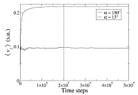Running average of the total flow velocity along the direction of the external force, $\left \langle v_{z} \right \rangle$, as function of the simulation time-steps.

The velocity profiles developed by the simulated systems were calculated using 4 x 10 ⁵ simulation steps after thermalization. With the purpose of calculating such velocity profiles, we sort the simulated particles according to their positions along x-axis every time-step. We calculated the average of the velocity along the z-axis of those particles located in parallel layers of width a. Then, the a final averaging process was conducted over the afore mentioned 4 × 10 ⁵ time-steps.

We shall present here the results obtained from the application of the algorithm described in the previous section. With this purpose it will be convenient to show first in section 4.1, those results obtained when the confining forces are applied according to the simulation scheme I, [Eq. 6] with $F_{||} = 0$. Subsequently in section 4.2 we will estimate the values of $F_{||}$ that must be used in the simulation scheme II, in order to achieve confining walls with no slip boundary conditions.

First, we notice that the velocity profile expected for the geometry described in the previous section is the classical plane Poiseuille flow (Landau and Lifshitz, 1959), which will be cast in the form

where v is the kinematic viscosity of the fluid and D_x is the effective distance between the parallel plates, i.e., the total distance between the planes of zero flow velocity.

In the first stage of our numerical analysis we pursued to verify that our implementation gives to the correct velocity flow, as they are given by [Eq. 9With this purpose, we conducted experiments in which α took twelve different values uniformly distributed within the range α ∈ [15° , 180° ]. It should be mentioned that for small values of the collision angle, the simulated system is expected to behave close to the so-called gas regime, in which contributions to the material properties of the fluid arising from streaming (kinetic) dynamics dominate over contributions due to collisions (Kapral, 2008; Gompper et al., 2009). On the opposite case, for values of α close to 180° , the dynamics of the simulated fluid is expected to be in the so-called liquid regime, where collisional effects are larger and dominate over kinetic effects. Consequently, in our numerical experiments we were able to explore the complete range of behaviors exhibited by MPC fluids. Moreover, for each selected collision angle, experiments were performed with 51 different values of g uniformly distributed in the range $g \in \left [ 0,0.5a/u_{t}^{2} \right ]$. For brevity, the units of the force per unit mass will be omitted in the following. Notice that this gives a total of 612 numerical experiments that were performed to test the applicability of the proposed technique.

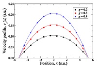Typical velocity profiles obtained from simulations of confined MPC fluids, performed according with scheme I at collision angle α = 180° . Symbols correspond to numerical results while continuous curves have been obtained from a quadratic fit.

We observed that in all the performed experiments a velocity profile was established in the system that could be very well adjusted by a parabolic fit. This situation is illustrated in Fig. 4 where we have plotted three typical velocity profiles, obtained from simulations carried out at the fixed collision angle α = 180° , and the external force fields g= 0.2,0.3, and $0.4a/u_{t}^{2}$ . These profiles were calculated as the time average of the z component of the center of mass velocity of the MPC cells, evaluated at different x positions inside the simulation cell. The continuous curves presented in Fig. 4 were obtained from a nonlinear fit of the simulation results assuming a quadratic relation between v_z and x of the form $v_{z}=a_{1} \left ( \left ( \tilde{D}_{x}/2 \right )^{2} - x^{2} \right )$, where a₁ and $\tilde{D}_{x}$ are the adjustable parameters, $\tilde{D}_{x} = \tilde{D}_{x} (\alpha ,g)$ being the experimentally estimated value of $\tilde{D}_{x}$ for given α and g. Our numerical results show that variations of $\tilde{D}_{x}$ with the external force field are not significant, as it can be seen in the case illustrated in Fig. 4, but $\tilde{D}_{x}$ was found to strongly depend on the collision angle. Thus, we obtained a final estimation of D_x for a given α, $\tilde{D}_{x}(\alpha )$, by averaging over the set of values of g. We present in Fig. 5 the result of this analysis where $\tilde{D}_{x}$ is plotted as function of the collision angle. In that figure, the horizontal dashed line represents the location of the interaction surface, $L_{x} /2$.

It is interesting to look at Fig. 5 that the estimated distance $\tilde{D}_{x}$ does not coincide with the location of the confining walls, i.e., $\tilde{D}_{x} \ne L_{x}$. This implies that the hydrodynamic flow does not vanish at the surface of fluid-solid interaction and that the simulation scheme I yields boundaries with partial slip, an effect that can be interpreted in terms of an apparent viscosity contribution at the neighborhood of the confining surfaces (Gompper et al., 2009; Winkler and Huang, 2009). We found experimentally that for values of the collision angle in the range α ∈[60° , 180° $\tilde{D}_{x} > L_{x}$; while for smaller values of α, i.e., α ≤ 60° ,$\tilde{D}_{x}$ was found to be smaller than $L_{x}$. Accordingly, we can conclude that in the regime where kinetic effects dominate, the force exerted by the confining surfaces makes the MPC fluid move in the opposite direction to the external force $\underset{g}{\rightarrow}$ . This effect can be explained by noticing that when 𝛼 is small, MPC particles may travel large distances without changing their velocities appreciably. Accordingly, particles inside the simulation box, but far from the interaction region, with rather large velocities along the direction of $-\underset{g}{\rightarrow}$ , are able to collide with the wall, from where they are rejected with large velocities pointing mainly in the direction of −𝑔 . These rejected particles drag the fluid at boundary walls and are responsible for the aforementioned backward motion. In section 4.2, we will discuss how the partial slip at the confining walls can be eliminated.

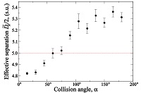Estimated effective system size, $\tilde{D}_{x} /2$, as function of the collision angle 𝛼 in simulations performed according to scheme I.

We used the results of the numerical experiments described previously to estimate the viscosity of the simulated MPC fluid, as function of the collision angle 𝛼. With this purpose, it can be verified according to [Eq. 9], the average velocity produced by the external force is

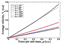Average velocity induced by external force fields, $\underset{g}{\rightarrow}$ , with different magnitude in MPC fluids confined according with scheme I. Symbols are used to represent numerical results. The black line shown in the case α=15° corresponds to a fit of the experimental data in the range g=∈ $\left [ 0,0.4a/u_{t}^{2} \right ]$, obtained from a simple least squares method.

We used [Eq. 10] to estimate v(α) as follows. We measured $\underset{v}{\rightarrow}_{z}$ for each performed experiment as the time average of the 𝑧 component of the center of mass velocity of the MPC cells, calculated over the whole simulated system. In Fig. 6 we present the results of such measurements. For simplicity, there we have only included the results for some selected values of the collision angle, namely α= 15° , 45° , 75° , 105° , 135° , and 165° . It can be observed that for small values of the external force, all the experiments show that $\underset{v}{\rightarrow}_{z}$ increases linearly with g, as it is expected from [Eq. 10]. In Fig. 5 it is also shown that the linear relation between the average velocity and the external force is broken for large values of the latter, $g \ge 0.4a/u_{t}^{2}$ . For simplicity, this situation is illustrated in Fig. 6 only for the case α= 15° , however, it is indeed observed for the complete set of numerical experiments. The departure of $\underset{v}{\rightarrow}_{z}$ from the linear behavior implies that the proposed technique for confining MPC fluids might lead to a stress tensor that depends on the external force.

This effect can be explained by taking into account that under confinement, the stress tensor of the fluid has a kinetic contribution due to its interaction with the walls (Winkler and Huang, 2009). The stress at the wall corresponding to our implementation could be obtained from the average of the momentum exchange occurring during the streaming step. Let t_q and t_q + Δt denote the times at which two consecutive SRD collisions take place, and consider a fluid particle that collides with the wall at time t_q+ δt, with 0 ≤ δt ≤ Δt The total momentum change of this particle, relative to the center of mass velocity of the fluid from where it comes, is

Notice that in our implementation particles interacting with the wall, are not affected by the force field $\underset{g}{\rightarrow}$. Then, the last term in the previous equation represents the acceleration of the fluid in the bulk phase with respect to the particles absorbed by the wall. This acceleration generates a contribution to the stress that depends on the external force per unit mass g, as it has been found in our simulations. Nevertheless, it is clear from Fig. 6 that this effect could be neglected if simulations are kept in the limit of small values of the external force. We restricted ourselves to consider this case and approximated the results presented in Fig. 6 by the simple numerical relation $\underset{v}{\rightarrow}_{z}= s(\alpha )g$, where the slope s(α) was obtained by the method of least squares, applied only over the limited range $0< g \le 0.4a/u_{t}^{2}$ . This result can be used in combination with [Eq. 10] to give the estimation of the kinematic viscosity, $\underset{v}{\rightarrow}$̃, according to $\underset{v}{\rightarrow}=\underset{D}{\rightarrow}_{x}^{2}(\alpha )/12s(\alpha )$.

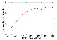Estimated viscosity coefficient of the confined MPC fluid, $\hat{v}$, as function of the collision angle α. Symbols with error bars are the results from simulations.

We present in Fig. 7 the results obtained from this analysis, where the estimated viscosity of the MPC fluid was calculated for the whole set of values of the collision angle used in our simulations. It can be observed from Fig. 7 that $\underset{v}{\rightarrow}$ increases rapidly for small values of α, but it is stabilized and presents no significant variations for values of α close to 180°. The empirical function $\underset{v}{\rightarrow}(\alpha )$ was approximated by a polynomial expansion of the form

where α must be given in radians and the constant coefficients k_i, i= 0,1,2,3,4, were estimated from a nonlinear fitting procedure of the experimental data. They turned out to have the explicit values k₀ = 0.117266, k₁ = 0.773052,k₂ = 0.184448, k₃ = −0.232476, and k₄ = 0.042175. This approximation is represented by the continuous curve in Fig. 7.

It is worth stressing that the viscosity coefficient of the simulated fluid described by [Eq. 12] and Fig. 7, differs from the viscosity calculated in other models and simulations of MPC (see, e.g., [Eq. 32] and [Eq. 39] in (Gompper et al., 2009)). The reason for this discrepancy is that under confinement, the stress on the MPC fluid has contributions due to the interaction with the walls. This contribution modifies the total stress of the fluid and produces the particular behavior of 𝜈̃ observed in our experiments. In this sense, the viscosity coefficient estimated empirically by [Eq. 12] can be considered as an effective parameter valid to describe the flow produced in the simulated system. Subsequently, in section 4.3, we will show that the values of the effective viscosity obtained empirically are very well adjusted by the expected analytical expression of the viscosity in the liquid-like regime of MPC and that, at least in such regime, the velocity profile obtained from our implementation approaches the analytical reference Poiseuille flow.

We carried out a comparison of the results of simulations with the classical Poiseuille formula, [Eq. 9], in which we used the values of $\tilde{v}(\alpha )$ and $D_{x}(\alpha )$ estimated according to the procedure described earlier. This comparison is shown in Fig. 8 for simulations performed with collision angles α= 15° , 90° , and 180° , and external forces per unit mass g = 0.1,0.2, and $0.4a/u_{t}^{2}$ . It can be observed in Fig. 8 that the proposed model is very satisfactory to describe the behavior of the system in the whole set of selected parameters.

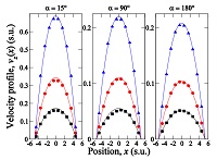Plane Poiseuille flows induced by the application of external forces with different magnitudes $g=0.1a/u_{t}^{2}$ (squares), $g=0.2a/u_{t}^{2}$ (circles), and $g=0.4a/u_{t}^{2}$ (triangles), in simulations of confined MPC fluids carried out according to scheme I with three different collision angles α.

Finally, it is worth stressing that in order to characterize the flow produced in our numerical implementation and to relate it with the corresponding to a physical fluid, hydrodynamic dimenssionless parameters can be used. In particular, we will consider the Reynolds number, Re, which for a given flow quantifies the relevance of the inertial force with respect to the viscous effects. For plane Poiseuille flow, Re can be written in the form

$$Re=\frac{\tilde{v}_{z}L_{z}}{v}$$

Therefore, it can be appreciated from the results presented in Figs. 5 and 6, that our simulations, corresponds to flows with a maximum Reynolds number Re ≅15. At the end of the following section we will present the results of simulations with larger values of Re.

It has been shown in section 4.1 that the simulation scheme I, in which confining forces act in the opposite direction of the velocity of the incoming MPC particles, yields partial slip boundary conditions. This indicates that an additional stress at the boundary needs to be added in order to restore no slip conditions at the confining surfaces. The additional stress might be generated from the force $\underset{F}{\rightarrow}_{||}$appearing in [Eq. 6]. In this work, we followed a numerical approach to determine the strength of the force $\underset{F}{\rightarrow}_{||}$ that must be applied in simulations to obtain stick boundary conditions. More precisely, we implemented an optimization procedure in which simulations at fixed α and g were carried out with different values of $F_{||}$ . We considered a steepest descendant method in which $F_{||}$ varied until we observed that the magnitude of the average velocity of the MPC fluid at the location of the confining surfaces, $x=\pm L_{x}/2$, was smaller than a fixed error value ε= 0.001. We performed this procedure for the whole set of values of the collision angle α, and for the following eight values of the external force per unit mass g = 0.05,0.10,0.15, … ,$0.4a/u_{t}^{2}$ 2 .

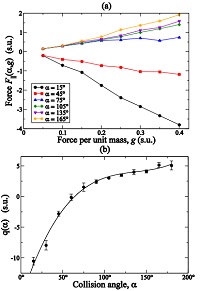(a) Magnitude of the parallel force, $\underset{F}{\rightarrow}_{||}=F_{||}\hat{e}_{z}$ (see [Eq. 6]), that must be applied in simulations of confined MPC fluids in order to restore stick boundary conditions. $F_{||}$ as function of g is well fitted by a linear relation $F_{||}=q(\alpha )g$. (b) Parameter $q(\alpha )$ as function of the collision angle.

Our results are presented in Fig. 9 (a). They show that $F_{||}$ can be very well approximated by the linear relation

where $q(\alpha )$ is the slope of the line obtained at a fixed value of α. We conclude that, with the purpose of simultaing surfaces with no slip boundary conditions, the fluid-solid interaction must occur with local walls whose inclination depart from that given by the incoming velocity of the particles by an amount proportional to the force field acting on the fluid phase

We estimated the values of $q(\alpha )$ using the method of least squares and plot the results in Fig. 9 (b). There, the continuous curve was obtained by a polynomial regression that fits the experimental data according to

where the constants h₀, h₁, h₂ and h₃ were found to have the values, in simulation units, h₀ = −16.81, h₁ = 24.14, h₂ = −9.66 and h₃ = 1.34. Regard that in [Eq. 14], α is given in radians, although it is plotted in grads in Fig. 9 (b).

Equations [Eq. 13] and [Eq. 14] represent the main results of this section. They can be used to determine the value of $F_{||}$ that must be applied in a numerical experiment, performed at given α and g, in order to achieve stick boundary conditions. In other words, thanks to the considerable amount of performed simulations, in future experiments it will be unnecesary to apply the steepest descendant procedure to obtain stick boundary conditions, but instead [Eq. 13] and [Eq. 14] can be used to obtain flows whose velocities at the confining planes will be smaller than the error parameter ε.

In order to test the applicability of our methodology, we carried out experiments according to the simulation scheme II, in which the force $F_{||}$ given by [Eq. 13] and [Eq. 14] was applied. The selected parameters were α= 30° , 135° and $g=0.2a/u_{t}^{2}$ . The results are compared with those given by the simulation scheme I in Fig. 10. There, the vertical axes coincide with the location of the surfaces where the fluid-solid interaction takes place. It can be noticed that stick boundary conditions are achieved by the implementation of scheme II. In other words, slip at the boundary is indeed removed by the application of such procedure. Finally, it can be seen that the viscosities of the fluids simulated by schemes I and II exhibit no significant differences.

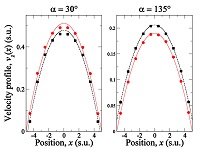Comparison between the velocity profiles obtained from simulation schemes I (squares, dashed curves), and II (circles, continuous curves).

As it has been stressed in subsection 4.1.2, the analysis carried out up to now is based on an empirical estimation of the viscosity of the simulated fluid. This estimation implicitely contains contributions to the stress tensor of the fluid originated by the application of the force $f_{||}$, by the incorporation of the virtual particles, and by the velocity rescale carried out in the thermostatting step. In the present section we will exhibit that in the limit of liquidlike behavior, these contributions are small, and that the viscosity of the simulated flow can be approximated by that expected from the analytical expressions obtained for the SRD-MPC implementation, in which is written in the form $v=v^{\textrm{col}}+v^{\textrm{kin}}$, with (Gompper et al, 2009)

and

With this purpuse, we implemented 5 additional experiments where flows were promoted by a pressure gradient with magnitude $g=0.2a/u_{t}^{2}$ , in an MPC fluid characterized by the parameters α= 135° , N_p = 5, and Δt= 0.05. As it was the case before, we considered the values k_BT = 1, and m= 1. For such parameters the theoretical expected value of the viscosity of the fluid is, according to [Eq. (15)] and [Eq. (16)], ν = 1.55. The difference between the new experiments and those considered in the previous sections is that the size of the system was varyied. In the present case, simulations were performed with L_y=L_z=32a, and L_x= 8, 12,16,18 and 20a. We carried out the procedure for achieving non-slip boundary conditions described in section 4.2 in each one of the considered cases, and estimated the empirical viscosity of the fluid by a non-linear fitting procedure. We observed that this quantity depends on the distance between the confinning walls L_x . We summarize in Table I the results obtained for this last series of experiments. We notice that although for our implementation the kinematic viscosity is indeed sizedependent, it seems to tend to a stable value, v= 1.61, for relatively large systems $L_{x}\ge 16a$. This value differes in 3.9% from the expected from [Eq. (15)] and [Eq. (16)]. A deviation of this magnitude could be expected since, as it has been described in section I, it has been reported that the use of the simple local rescaling thermostat interferes with the flow and could produce variations in the apparent viscosity of the fluid that could be as large as 5%.

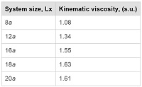Kinematic viscosity obtained in numerical experiments of MPC fluids confined by walls with different separation.

In Fig. 11 we present a comparison between the velocity profiles obtained numerically in the cases of systems with sizes L_x= 18a, and L_x= 20a, with those expected theoretically for non-slip boundary conditions, calculated from the classical Poiseuille formula, [Eq. (9)], in which the kinematic viscosity was estimated with [Eq. (15)] and [Eq. (16)]. With the purpose of obtaining a more detailed description of the velocity profiles than the one presented in sections 4.1 and 4.2, in the new series of experiments, these profiles were calculated from averages over particles located within layers of width a/4, parallel to the yz-plane. It can be observed that due to the discrepancy in the values of the numerical and theoretical viscosities, the experimental flow profile (symbols) deviates from the theoretical model. In addition, the insets in Fig. 11 show that the numerical profiles exhibit differences with their theoretical counterparts close to the walls, which could be expected since in our numerical procedure no-slip boundary conditions are obtained in an approximated fashion by the optimization procedure described in sections 3 and 4.2.

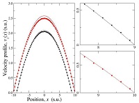Comparison between the velocity profiles obtained from simulation in systems of sizes Lx = 18a (black circles), and Lx= 20a (red squares). The continuous curves are the corresponding theoretical Poiseuille flows of reference

We have presented a methodology for simulating plane Poiseulle flow in MPC. This methodology is new, in the sense that it combines diverse procedures that have not been applied together to study the confinement this kind of fluids. First, we consider the introduction of an explicit repulsive potential between the simulated fluid particles and the particles of a solid physical wall, a procedure that was introduced by us in(A. AyalaHernandez and H. Híjar, 2016). The most important feature of this formalism, summarized in [Eq. 2] and [Eq. 3], is that the microscopic details of the confinement palne walls have been averaged and reduced to its local geometry. This characteristic of the proposed method will be exploited in subsequent publications, where it will be applied in simulations of MPC fluids confined between concentric cylindrical channels. In addition, it is worth stressing that the formalism used in this work is alternative to some other existent in the literature that have been used for MD and Dissipative Particle Dynamics(Spijker et al., No5; Pivkin and Karniadakis, 2005).

Then, we discussed how the problem of confinement of MPC fluids by means of explicit forces presented some difficulties that are also found when these fluids are confined by hard walls methods. In particular, it was necessary to propose an algorithm for the application of [Eq. 2] and [Eq. 3], that included a procedure for the introduction of virtual particles at the collision step. Although diverse techniques for incorporating virtual particles in MPC are available in the literature (Lamura et al., 2001; Lamura and Gompper, 2002; Winkler and Huang, 2009), they have not been used before in simulations of MPC particles in the presence of physical walls.

Finally, an implementation for eliminating partial slip at the surface of fluid-solid interaction was incorporated. In this procedure, an additional tangential force acting on the particles interacting with the solid wall was applied. The strength of this force was determined empirically from the results of a large number of numerical experiments. Although this procedure resembles one used in other coarse-grained computer simulations of fluids (Lamura and Gompper, 2008), we stress that our work is the first that considers the effects of tangential forces in MPC simulations. We would like to emphasize also, that this procedure for achieving no-slip boundary conditions differs from the one used in(A. Ayala-Hernandez and H. Híjar, 2016), where velocity at the solid surface was controlled by varying the momentum of the virtual particles.

We have shown that the combination of these techniques simulates the correct velocity profile expected for no slip boundry conditions. Modifications of the present algorithm could be introduced that would allow us for simulating solid surfaces with arbitrary slip coefficient and moving confining walls. These problems are under current research.

A final comment concerns the comparison of the computational performance of the proposed method with those existent in the literature that are also used to simulate hydrodynamic flow in MPC. We have not carried out such comparison in the present work, since our interest was focused in testing the validity of the proposed technique. However, it can be anticipated that our implementation will have an inferior computational efficiency when compared with, e.g., the hard-wall method for simulating plane Poiseuille flow in MPC, due to the computational cost that must be paid during the streaming step by the application of the MD integration scheme. Nevertheless, our method has the property of yielding simulations that are in fact closer to real situations than those produced by hardwall schemes, because confinement of fluids by solids must always result from an explicit potential existing between their microscopic components and not from an interaction of the hard wall type.

H. Híjar thanks Dr. G. Sutmann from FZ-Jülich for useful discussions and Universidad La Salle for financial support under grant NEC-04/15.

References

• Ali, I.,Marenduzzo, D., and Yeomans, J. Dynamics of polymer packaging. (2004).J. Chem. Phys.,121:8635.
• Allahyarov, E. and Gompper, G. (2002). Mesoscopic solvent simulations: Multiparticlecollision dynamics of three-dimensional flows.s.Phys. Rev. E, 66:036702.
• Ayala-Hernández, A. (2016).Simulación Mesoscópica de fluidos confinados por fronteras sólidas. (Master’s thesis, La Salle University Mexico) (in Spanish)
• Ayala-Hernández, A. and Híjar H. (2016). Simulation of Cylindrical Poiseuille Flow in Multiparticle Collision Dynamics using explicit Fluid-Wall confining forcesRev. Mex. Fis. 62:73.
• Belushkin, M., Winkler, R. G. and Foffi, G. (2011). Backtracking of colloids: A multiparticle collision dynamics simulation studyJ. Phys. Chem. B, 115:14263.
• Bolintineanu, D. S., Lechman, J. B., Plimpton, S. J., and Grest, G. S. (2012). TPhys. Rev. E86:066703
• Fernández , J. and Híjar, H. (2015). Mesoscopic simulation of Brownian particles confined in harmonic traps and sheared fluids.Rev. Mex. Fis., 61:1.
• Frenkel, D. and Smith, B. (2002)Understanding Molecular Simulations: from Algorithms to Applications. Academic Press, San Diego.
• Gompper, G., Ihle, T. , Kroll, D. M., and Winkler, R. G. (2009). Multi-Particle Collision Dynamics: A particle-based mesoscale simulation approach to the hydrodynamics of complex fluids. Adv. Polym. Sci., 221:1–87.
• Griebel, M., Knapek, S., and Zumbusch, G. (2007)Numerical Simulation in Molecular Dynamics. Numerics, Algorithms, Parallelization, Applications Springer, Berlin Heidelberg
• Hansen, J. P. and McDonald, I. R. (1986).Theory of simple liquids, 2nd ed.Academic Press, London.
• Hecht, M., Harting, J., Ihle, T., and Hermann, H. J. (2005). Simulation of claylike colloids. Phys. Rev. E, 72:011408.
• Ackerman, B. (2014) “Obama’s Betrayal of the Constitution” in The New York Times Op-Ed, Friday, September 12, 2014, p. A31.
• Híjar, H. and A. Ayala-Hernandez (2016). Flow between concentric cylinders simulated with multiparticle collision dynamics. Rev. Mex. Fis. (In press).
• Híjar, H. and Sutmann, G. (2011). Hydrodynamic fluctuations in thermostatted multiparticle collision dynamics. Phys. Rev. E,83:046708.
• Híjar, H. (2013). Tracking control of colloidal particles through non-homogeneous stationary flows. J. Chem. Phys., 139:234903.
• Híjar, H. (2015). Harmonically bound Brownian motion in fluids under shear: FokkerPlanck and generalized Langevin descriptions.Phys. Rev. E, 91:022139.
• Huang, C. C., Chatterji, A., Sutmann, G., Gompper, G. and Winkler, R. G. (2010). Celllevel canonical sampling by velocity scaling for multiparticle collision dynamics simulations, J. Comput. Phys., 229:168.
• Huang, C. C., Varghese, A., Gompper, G., and Winkler, R. G. (2015). Thermostat for nonequilibrium multiparticle collision dynamics simulations.s. Phys. Rev. E, 91:013310.
• Ihle, T. and Kroll, D. M. (2001). Stochastic rotation dynamics:a Galilean-invariant mesoscopic model for fluid flow.Phys. Rev. E, 63:020201.
• Ihle, T. and Kroll, D. M. (2003). Stochastic Rotation Dynamics II. transport coefficients, numerics, and long-time tails.Phys. Rev. E, 67:066706.
• Imperio, A., Padding, J. T. and Briels, W. (2011). Force calculation on walls and embedded particles in multiparticle-collision-dynamics simulations, Phys. Rev. E 83:046704.
• Inoue, Y., Chen, Y., and Ohashi, H. (2002). Development of a simulation model for solid objects suspended in a fluctuating fluid. J. Stat. Phys., 107:85.
• Moncho Jordá A., Louis, A. A., and Padding, J. T. (2010). Effects of interparticle attractions on colloidal sedimentation. Phys. Rev. Lett., 104:068301.
• Moncho Jordá, A., Louis, A. A., and Padding, J. T. (2012). How Peclet number affects microstructure and transient cluster aggregation in sedimenting colloidal suspensions.J. Chem. Phys., 136:064517.
• Kapral, R. (2008). Multiparticle Collision Dynamics: Simulation of complex systems on mesoscales. Adv. Chem. Phys., 140:89
• Kikuchi, N., Gent, A., and Yeomans, J. M. (2002). Polymer collapse in the presence of hydrodynamic interactions. Eur. Phys. J. E 9:63.
• Kikuchi, N., Ryder, J. F., Pooley, C. M., and Yeomans, J. M. (2005). Kinetics of the polymer collapse transition: The role of hydrodynamics. Phys. Rev. E, 71:061804.
• Lamura, A., Gompper, G., Ihle, T., and Kroll, D. M. (2001). Multi-particle collision dynamics: Flow around a circular and a square cylinder. Europhys. Lett., 56:319.
• Lamura, A. and Gompper, G. (2002). Numerical study of the flow around a cylinder using multi-particle collision dynamics. Eur. Phys. J. E, 9:477.
• Lamura, A. and Gompper, G. (2008). Tunable-slip boundaries for coarse-grained simulations of fluid flow. Eur. Phys. J. E, 26:115.
• Landau, L. D. and Lifshitz, E. M. (1959).Fluid Mechanics, 2nd revised English version. Pergamon, London.
• Lee, S. H. and Kapral, R. (2004). Friction and diffusion of a Brownian particle in a mesoscopic solvent.J. Chem. Phys., 121:11163.
• Malevanets, A. and Kapral, R. (1999). Mesoscopic model for solvent dynamics.J. Chem. Phys., 110:8605.
• Malevanets, A. and Kapral, R. (2000). Solute molecular dynamics in a mesoscale solvent. J. Chem. Phys., 112:7260.
• Malevanets, A. and Yeomans, J. M. (1999). Dynamics of short polymer chains in solution. Europhys. Lett., 52:231.
• Noguchi, H. and Gompper, G. (2005). Dynamics of fluid vesicles in shear flow: Effect of membrane viscosity and thermal fluctuations.Phys. Rev. E, 72:011901.
• Padding, J. T. and Louis, A. A. (2004). Hydrodynamic and Brownian fluctuations in sedimenting suspensions.Phys. Rev. Lett., 93:220601.
• Padding, J. T. and Louis, A. A. (2006). Hydrodynamic interactions and Brownian forces in colloidal suspensions: Coarse-graining over time and length scales.Phys. Rev. E, 74:031402.
• APivkin, I. V. and Karniadakis, G. E. (2005). A new method to impose no-slip boundary conditions in dissipative particle dynamics.J. Comp. Phys., 207:114.
• Pooley, C. M. and Yeomans, J. M. (2005). Kinetic theory derivation of the transport coefficients of stochastic rotation dynamics. J. Phys. Chem. B, 109:6505, 2005.
• Ackerman, B. (2014) “Obama’s Betrayal of the Constitution” in The New York Times Op-Ed, Friday, September 12, 2014, p. A31.
• Ripoll, M., Mussawisade, K., and Winkler, R. G. (2004). Low-Reynolds-number hydrodynamics of complex fluids by multi-particle-collision dynamics.Europhys. Lett., 68:106
• Spijker, P., Eikelder, H. M. M., Markvoort, A. J., Nedea, S. V., and Hilbers, P. A. J. (2008). Implicit Particle Wall Boundary Condition in Molecular Dynamics. Engineering Science, 222:855–864, No.5.
• Tüzel E., Strauss, M., Ihle, T., and Kroll, D. M. (2003). Transport coefficients for stochastic rotationdynamics in three dimensions. Phys. Rev. E, 68:036701.
• Winkler, R. G. and Huang, C. C. (2009). Stress tensors of multiparticle collision dynamics fluids. J. Chem. Phys., 130:074907.
• Withmer, J . K. and Luijten, E. (2010). Fluid-solid boundary conditions for multiparticle collision dynamics. J. Phys.: Condens. Matter, 22:104106.
• Yeomans, J. M. (2006). Mesoscale simulations: Lattice Boltzmann and particle algorithms. Physica A, 369:159.